In this blog, I will be explaining the task we were working on for the last 3-4 weeks. It will take you on a journey of optimizations from million graph traversals in building the database to just a few traversals in the end. Also, we will be covering the new architecture for the upcoming version of the Linked Commons and the reason behind the change.

Where does it fit?

So far the Linked Commons was using a tiny subset of the data available in the CC Catalog. One of the primary targets of our team was to update the data. If you observe closely all tasks so far starting from adding "Graph Filtering Methods" to "Autocomplete Feature". These were actually bringing us closer towards this task. i.e. the much-awaited "Scale the Data of Linked Commons". We aim to add around 235k nodes and 4.14 million links into the Linked Commons project from around 400 nodes and 500 links in the current version. This drastic addition of new data is one of its kind, which makes this task very challenging and exciting.

Pilot

The raw CC Catalog data cannot be used directly in the Linked Commons. Our first task involves processing it, which includes removing isolated nodes, etc. You can read more about it in the data processing series blog written by my mentor Maria. After this, we need to build a database which stores the "distance list" of all the nodes.

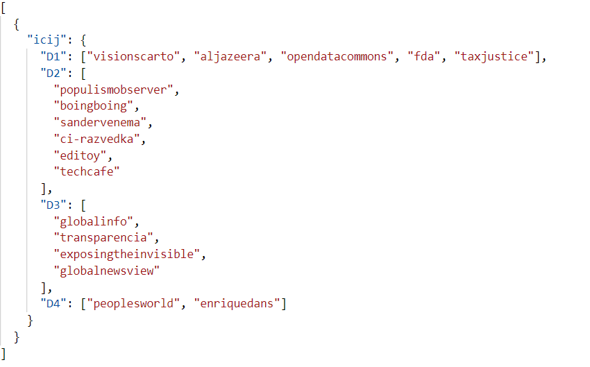
What is "distance list"?

Distance List is a method of graph representation. It is similar to Adjacency List representation of graphs but instead of storing data of just immediate neighbouring nodes, "distance list" groups all vertices based on their distance from the root node and stores this grouped data for every vertex in the graph. In short, "distance list" is a more general form of the Adjacency List representation.

To build this "distance list", we created a script for this, let’s name it build-dB-script.py, which uses the Breadth-First Search(BFS) algorithm on every node to traverse the graph and gradually build this distance list. The filtering nodes feature of our web page connects to the server, which uses the aforementioned database and serves a smaller chunk of data.

Problem

Now that we know where the build-dB-script is used, let’s discuss the problems with it. The new graph data we are going to use is enormous and is in millions. A full traversal of a graph with million nodes, million times is very slow. Just to give some helpful numbers, the script was taking around 10 minutes to process a hundred nodes. Assuming the growth is linear(in the best case), it will take more than 15 days to complete the computations. It is scary, and thus, optimizations in the build-dB-script are the need of the hour!!

Optimizations

In this section, we will talk of the different versions of the build database script, starting from the brute force BFS method.

The brute force BFS was the most simple and technically correct solution, but as the name suggests it was slow. In the next iteration, I stored the details of last n nodes, 10 to be precise and performed the same old BFS. It was faster but it had a logic error. Say, there is a link from a node to an already visited/traversed node. The script was not putting all the nodes which could have been explored from this path. After a few more leaps from Depth-first Search, to Breadth-first search, and other methods, eventually with the help of my mentors, we built a new approach - "Sequential dB Build".

To keep this blog short, I won’t be going too much into implementation details, but here are some of the critical points.

Key points of the Sequential dB Build:

• It was the fastest of all the predecessors and reduced the script timing significantly.
• In this approach, we aimed to build the all distance list of [1, 2, 3,... ., k-1] before building kth distance list.

Unfortunately, still, it was not enough for our current requirements. Just to give you some insights, the distance two list computation was taking around 4 hours, and distance three list computation was taking 20+ hours. It shows that all these optimizations were not enough and were incapable of handling this big dataset.

New Architecture

As the optimizations in "build-dB-scripts" weren’t enough, we started looking to simplify the current architecture. In the end, we want to have a viable product which is scalable to this massive data. Although we are still not dropping the multi-distance filtering, we will continue our research on it and hopefully will have it in Linked Commons 3.0. 😎

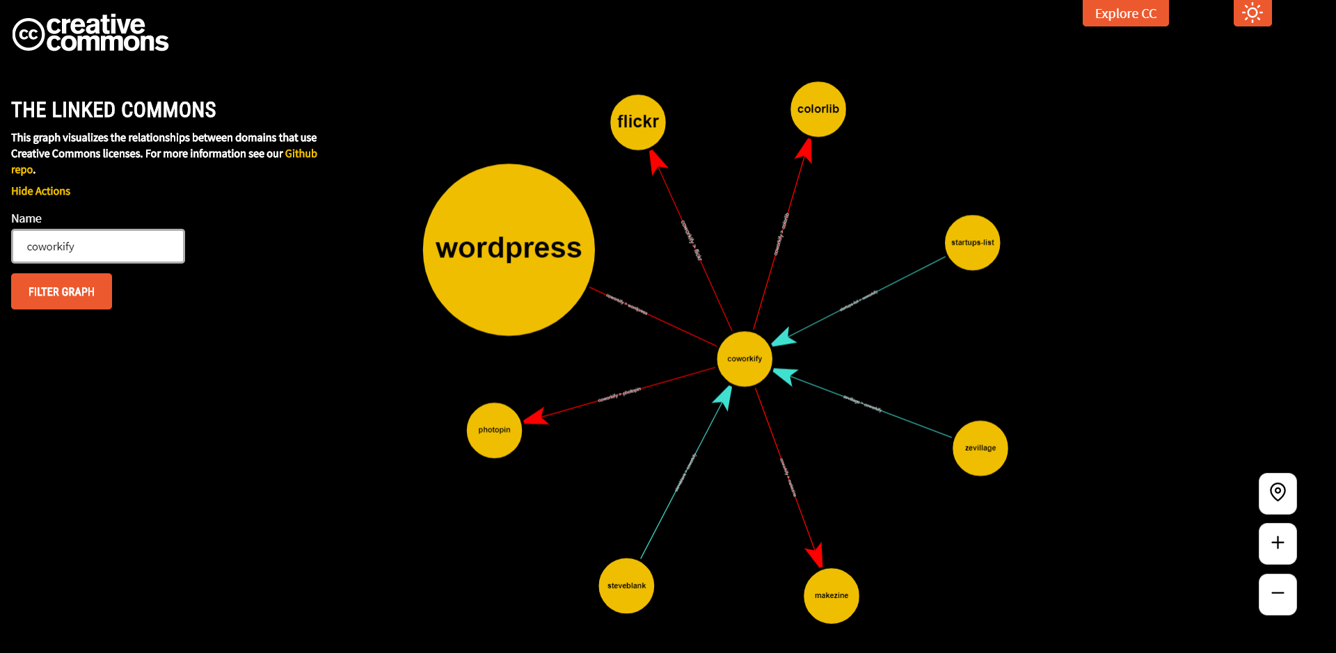
For any node, it is more likely that any person would wish to know the immediate neighbours who are linking to some arbitrary node. Nodes at a distance greater than one exhibits very less information on the reach and connectivity of the root node. It was because of this we decided to change our current logic of having the distance list up to 10; instead, we reduced it to 1 and also stored the immediate incomming nodes list (Nodes which are at distance 1 in the transpose graph).

This small change in the design simplified a lot of things, and now the new graph build was taking around 2 minutes. By the time I am writing this blog we have upgraded our database from shelve to MongoDB where the build time is further reduced. 🔥🔥

Conclusion

This task was really challenging and I learnt a lot. It was really mesmerizing to see the Linked Commons grow and evolve. I hope you enjoyed reading this blog. You can follow the project development here, and access the stable version of linked commons here.

Feel free to report bugs and suggest features. It will help us improve this project. If you wish to join the our team, consider joining our slack channel. Read more about our community teams here. See you in my next blog! 🚀

*Linked Commons uses a more complex schema. The picture is just for illustration.